
| 일 | 월 | 화 | 수 | 목 | 금 | 토 |
|---|---|---|---|---|---|---|
| 1 | 2 | 3 | 4 | |||
| 5 | 6 | 7 | 8 | 9 | 10 | 11 |
| 12 | 13 | 14 | 15 | 16 | 17 | 18 |
| 19 | 20 | 21 | 22 | 23 | 24 | 25 |
| 26 | 27 | 28 | 29 | 30 | 31 |
- 알고리즘
- flame
- numpy
- NLP
- deep learning
- 딥러닝
- point cloud
- Threshold
- reconstruction
- level2
- cv2
- center loss
- 논문 구현
- 파이썬
- 임계처리
- transformer
- OpenCV
- re-identification
- Object Tracking
- Object Detection
- attention
- 3D
- Knowledge Distillation
- Computer Vision
- 자료구조
- Deeplearning
- 스택
- Python
- 프로그래머스
- 큐
- Today
- Total
공돌이 공룡의 서재
[구현] 퍼셉트론 Numpy로만 구현하기 / Implement Perceptron by using Numpy Only 본문
퍼셉트론을 tensorflow, keras, 또는 torch를 사용하지 않고 구현하려면 forwarding과 back propagation, activation function 등이 어떻게 이뤄지고 구성되어 있는지를 정확히 알고 있어야 한다. 수학을 공부할 때 모르는 개념이 있다면 증명을 한 번 해보듯이, 입문하는 분들이라면 해볼 만한 과제라고 생각한다.
딥러닝 모델 구현은 크게 다음과 같은 부분으로 나뉠 수 있다.
- 모델 설정 : node의 수, weight의 초기값, bias의 초기값, 등을 설정한다.
- 손실함수 : 손실 함수에 대한 미분으로 역전파를 할 수 있다.
- feed forward : 입력층 - 은닉층 - 출력층까지 값을 주는 것을 말한다
- 손실 함수 & back propagation : 층 사이의 최적의 weight를 찾아가는 과정이다.
- training : 적절한 epoch와 학습률을 설정하여 학습한다. 여러 종류의 optimizer가 사용된다.
- validation / test : 딥러닝 모델은 결국 학습한 데이터 외에 다른 데이터에도 잘 적용되는지 여부가 중요하다. 만약 학습용 데이터에는 높은 정확률을 보이는데 그 외 데이터에는 그렇지 않다면 과대 적합(overfitting), 정확도 자체가 형편없으면 과소 적합(underfitting)이라고 한다.
1. 단층 퍼셉트론 (Single-layer Perceptron)
Input과 Output은 임의로 다음과 같이 설정해보겠다.
| [0, 0, 1, 0] | [0] |
| [0, 0, 1, 1] | [0] |
| [0, 1, 0, 0] | [0] |
| [0, 1, 1, 1] | [0] |
| [0, 1, 0, 1] | [1] |
| [1, 0, 1, 0] | [1] |
| [1, 0, 1, 1] | [1] |
| [1, 1, 1, 1] | [1] |
Test 셋은 따로 두지 않겠다.
단층 퍼셉트론이므로 모델은 다음과 같이 만들어볼 수 있겠다. bias는 따로 두지 않겠다.
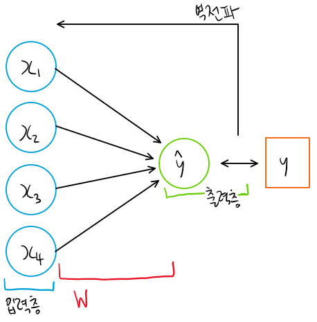
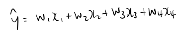
사실 단층 퍼셉트론의 경우 입력층에서 바로 출력층으로 가기 때문에 은닉층이 있다고 보기 힘들다. 다만 W, 즉 weight가 입력과 곱해지는 과정이 있다.
Activation Fuction으로는 sigmoid, Loss Function으로는 MSE를 사용하자. sigmoid(=s)의 경우, 역전파때 미분하면 s(1-s)가 됨을 알고 있자.
import numpy as np
# for visualization
import matplotlib.pyplot as plt
def forward_propagation(x, w):
# 각 input에 대해서 weighted_sum한 결과에 activation 함수까지 적용한 결과를 return한다
activation = []
for i in range(len(x)):
weighted_sum = w.T @ x[i]
act = 1 / (1 + np.exp(-weighted_sum))
activation.append(act)
activation = np.array(activation)
return activation
def backward_propagation(d_mse, prediction, inputs, weights, lr):
# loss function 에서 구한 d_mse를 이용한다. weights를 update한다.
weights += lr * d_mse.reshape(4, 1)
return weights
def loss_function(keys, prediction, inputs):
d_mse = 0
mse_loss = 0
for i in range(len(keys)):
# dEdW = 손실함수를 w로 미분한 것
dEdW = inputs[i] * (np.exp(-prediction[i]) / \
np.power((1 + np.exp(-prediction[i])), 2))
d_mse_i = (keys[i] - prediction[i]) * dEdW
d_mse += d_mse_i
mse_loss += np.power((keys[i] - prediction[i]), 2)
return (d_mse * 2)/len(keys), mse_loss * (1/(2*len(keys)))
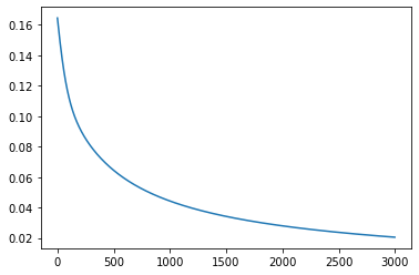
def visualization(data):
plt.plot(data)
def train(inputs, keys, weights, lr):
loss_list = []
for iter in range(3000):
prediction = forward_propagation(inputs, weights)
d_mse, mse_loss = loss_function(keys, prediction, inputs)
weights = backward_propagation(d_mse, prediction, inputs, weights, lr)
loss_list.append(sum(mse_loss))
result = np.where(prediction<0.5 , 0, 1)
# 결과 print
print(weights)
print(prediction)
print(result)
return loss_list
np.random.seed(1)
inputs = np.array([[0, 0, 1, 0],
[0, 0, 1, 1],
[0, 1, 0, 0],
[0, 1, 1, 1],
[0, 1, 0, 1],
[1, 0, 1, 0],
[1, 0, 1, 1],
[1, 1, 1, 1]])
# keys : ground truth
keys = np.array([[0, 0, 0, 0, 1, 1, 1, 1]]).T
# weight initialization
weights = 2 * np.random.random((4, 1)) - 1
#learning rate
lr = 0.05
loss_list = train(inputs, keys, weights, lr)
visualization(loss_list)
2. 다층 퍼셉트론(Multi layer Perceptron)
1번의 구조에서 Hidden layer를 추가해보자.
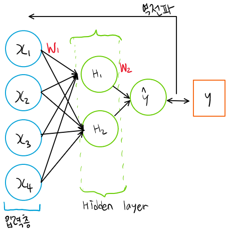
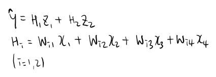
Weight인 W 와 Z는 각각 (2,4), (1,2)인 matrix가 되겠다. 역전파 식이 좀 더 복잡해진다. 텐서플로우나 토치같은 프레임워크를 사용하면 model을 class 형태로 구성하는 경우가 많으므로, 이런 흐름을 따라가 보겠다. activation function과 loss function은 위에서 했던 것과 똑같이 하겠다.
import numpy as np
import matplotlib.pyplot as plt

class MP:
    def __init__(self, inputs, labels, learning_rate, hidden_layers_shape):
        self.inputs = inputs
        self.labels = labels
        self.learning_rate = learning_rate
        self.hidden_layers_shape = hidden_layers_shape
        self.model_compose()
        self.history = [] # For visualization

    def model_compose(self):
        assert type(self.hidden_layers_shape) == list
        self.W = np.random.uniform(size=(self.hidden_layers_shape[0], self.hidden_layers_shape[1]))
        self.bias1 = np.random.uniform(size=(1, self.hidden_layers_shape[1]))
        self.Z = np.random.uniform(size=(self.hidden_layers_shape[1], self.hidden_layers_shape[2]))
        self.bias2 = np.random.uniform(size=(1, self.hidden_layers_shape[2]))

    def sigmoid(self, value):
        return 1 / (1+np.exp(-value))

    def sigmoid_d(self, value):
        return value * (1 - value)

    def forward(self):
        hidden_layer_output = self.sigmoid(self.inputs @ self.W + self.bias1)
        y_hat = self.sigmoid(hidden_layer_output @ self.Z + self.bias2)
        return hidden_layer_output, y_hat

    def back_propagation(self, h, o):
        """
        h = hidden_layer_output
        o = output
        """
        dLdo = o - self.labels.reshape(len(self.inputs),1)
        dLdZ= h.T @ (dLdo * self.sigmoid_d(o))
        dLdb2 = np.sum(dLdo * self.sigmoid_d(o), axis=0, keepdims=1)
        dLdW = self.inputs.T @ (dLdo * self.sigmoid_d(o) * self.Z.T * self.sigmoid_d(h))
        dLdb1 = np.sum(dLdo * self.sigmoid_d(o) * self.Z.T * self.sigmoid_d(h), axis=0, keepdims=1)
        self.W -= self.learning_rate * dLdW
        self.Z -= self.learning_rate * dLdZ
        self.bias1 -= self.learning_rate * dLdb1
        self.bias2 -= self.learning_rate * dLdb2

    def train(self, epochs:int):
        for epoch in range(epochs):
            h, o = self.forward()
            loss = np.mean(np.power((o- self.labels), 2)) / len(inputs)
            self.history.append(loss)
            self.back_propagation(h, o)

    def visualization(self):
        plt.plot(self.history)

    def check(self):
        h, o = self.forward()
        return h, o


 mp = MP(inputs=inputs, labels=labels, learning_rate = 0.05, hidden_layers_shape=[4 , 2, 1])
 inputs = np.array([[0, 0, 1, 0],
                   [0, 0, 1, 1],
                   [0, 1, 0, 0],
                   [0, 1, 1, 1],
                   [0, 1, 0, 1],
                   [1, 0, 1, 0],
                   [1, 0, 1, 1],
                   [1, 1, 1, 1]])

labels = np.array([[0], [0], [0], [0], [1], [1], [1], [1]])

mp.train(20000)

mp.check()

mp.visualization()
직접 구현하는데 있어서 back propagation 코드 작성이 생각보다 요구 사항이 많았다. 곱하는 행렬들 간의 차원들도 맞춰야 하고, 미분하는 식이 길어지다 보니 들어가야 할 변수나 값이 헷갈리긴 했다.
'딥러닝' 카테고리의 다른 글
| [논문 리뷰] XNOR - Net : classification using Binary CNN (0) | 2021.09.14 |
|---|---|
| [논문 리뷰] Adversarial attack: Universal Adversarial Perturbation (0) | 2021.09.05 |
| [개념] CNN : Convolution의 의미에 대하여 (0) | 2021.03.12 |


